We use the Gauss-Seidel iteration Method to solve the linear system equations. This method is named after the German scientist Carl Friedrich Gauss and Philipp Ludwig Seidel.
In an interconnected power system and its involved power system analysis the most fundamental and important tool is the Load Flow Analysis. So before diving any further deep into the Gauss-seidel Iteration method of Load flow analysis, let’s understand Load Flow Analysis.
What is Load Flow Analysis?
We can define Load Flow Analysis or Power Flow Analysis as a numerical analysis of the flow of electric power in any electrical system. It is more of an assessment of the steady-state conditions of the electrical system. The main goal of any load flow study is to determine the flow of power, current, voltage, real power, and reactive power in an electrical system under any load conditions. A load flow study is essential to ensure system voltages and current remain within safe limits during the design phase of a new project or when evaluating changes or additions to the existing electrical system.
Why do we need Load Flow Analysis?
Load flow studies or Power flow analysis is really helpful when making predictions by considering and analyzing various hypothetical situations related to electricity. For example, if we remove the transmission line from the system of a particular area, may it be for any reason, understanding whether the remaining line can serve or supply the load without exceeding its rated value. We can answer it well using a Load Flow Analysis.
Methods of Load Flow Analysis
- Gauss-Seidel System
This is considered to be one of the most common types of analysis. The advantages of the Gauss-seidel system involve simplicity in operation, the limited computational power required, and less time required to complete. However, it has a disadvantage such as its slow rate of convergence results in many iterations. Whenever a large power system with a greater number of buses is there, usually it increases the iterations.
- Newton-Raphson Method
In comparison to the Gauss-Seidel method, Newton Raphson is a more sophisticated method that uses quadratic convergence. The Newton Raphson method is more suitable for more complex situations.
The method takes fewer iterations to reach convergence and also takes less computer time. This method is less sensitive to complicating factors such as slack bus selection or regulating transformers, because of this reason this method is more accurate. It has very complicated programming, and therefore it requires a large computer memory. This is the disadvantage of Newton- Raphson method
- Fast Decoupled Load Flow System
This method is the most popular choice for the real-time management of power grids. The main advantage of this method is that it uses less computer memory. The calculation of this method is almost five times faster than the Newton-Raphson method. This method takes some assumptions to obtain fast calculations due to which it can be less accurate at times. It has a limited scope.
In this article, we will discuss the Gauss-Seidel Iteration method in detail.
Gauss-Seidel Method
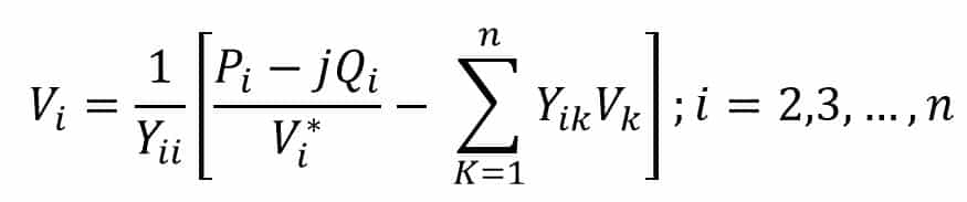
For solving the load flow solution with the Gauss-seidel method, we consider all the buses other than the slack bus as PQ buses. We can easily adapt this method to include PV buses as well. And as we know, the slack bus voltage is specified and all other ( n-1 ) bus voltages starting values of whose magnitudes and angles are assumed. Those values are then updated through an iterative process.
Gauss Seidel Algorithm
We shall consider where all buses other than slack are PQ buses.
- The active and reactive generations are allocated to the slack bus and are also allowed to vary during iterative computation, with the load profile known at each bus.
- YBUS is assembled by using the rule for self and mutual admittances, with the line and shunt admittances data stored in the computer.
- We assume a set of initial voltages to start the iterations. The voltage spread is not too wide in a power system, therefore it is a normal practice to use a flat voltage start I.e initially the voltages are set equal to (1 + j0) except the voltage of the fixed slack bus.
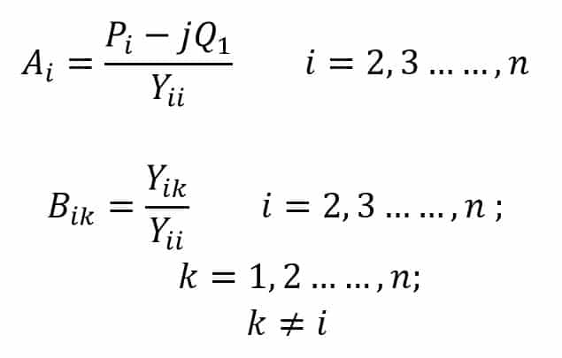
We can do some significant reduction in the computer time by performing some arithmetic operations that do not change with the iterations such as
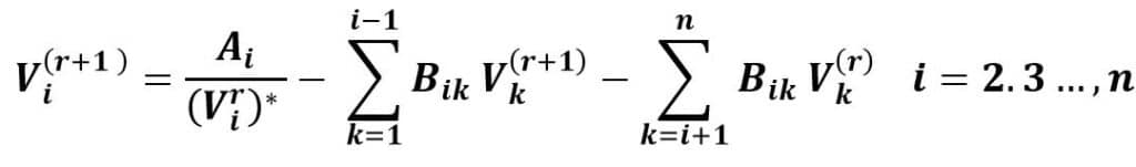
Now if we consider the (r+1)th iteration, the voltage equation becomes as below:
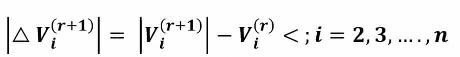
We continue this iteration till the bus voltage magnitude change between two back to back iterations is less than a certain tolerance for all bus voltages, i.e.
- We calculate the slack bus power along with V1 where it yields S1 = P1 + jQ1.
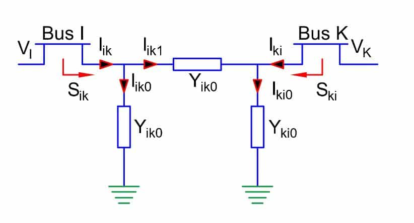
- The last step in the load flow analysis involves the computation of power flows on the various lines of the network. Suppose we consider the circuital representation of line connecting buses i and the line and transformers at each end with series impedance yik and two shunt admittances yik0 and yki0 .
Gauss-Seidel Method Explanation
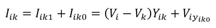
We can express the current injection from bus i into the line as:
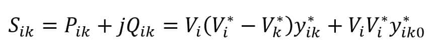
The power injection from bus i into the line is:
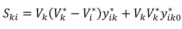
Similarly, power injection from bus k into the line is:
Now if we sum the power flows Sik + Ski , we get the power loss in the (i – k)th line. Similarly, we can compute total transmission loss by summing all the line flows.(i.e S ik + S ki for all i, k).
Note: We can also find the slack bus power by summing the power flows on the lines terminating at the slack bus.
Acceleration Factors in Gauss-Seidel Method
As we know, a large number of iteration is done to arrive at the specific convergence. It is possible to increase the rate of convergence by an acceleration factor. The acceleration factor reduces the number of alternations in the Gauss-Seidel method. The acceleration factor is a multiplier, and it enhances correction between the values of voltage in two successive iterations.
Let us consider the acceleration Factor for the ith bus.
- Vi(r) is the value of the voltage at the rth iteration.
- Voltage Value Vi(r + 1) is at the (r + 1)th iteration.
- Vi( accelerated)(r + 1) is the accelerated new value of the voltage at the (r+ 1) th iteration.
- r is the iteration count
- α is the accelerating factor
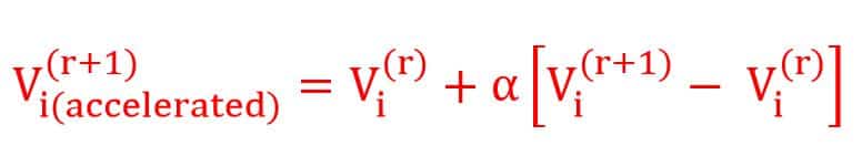
Then,
After calculating Vi(r + 1) at ( r + 1)th iteration, now, we calculate the value of the new estimated bus voltage Vi( accelerated)(r + 1) and this new value replaces the previously calculated value. We use real and imaginary components of the voltage different accelerating factors.
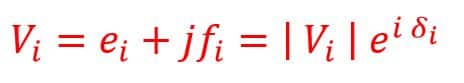
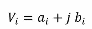
We can resolve Vi into real and imaginary components as
If α and β are the acceleration factor associated with ai and bi , then the equation is shown below.
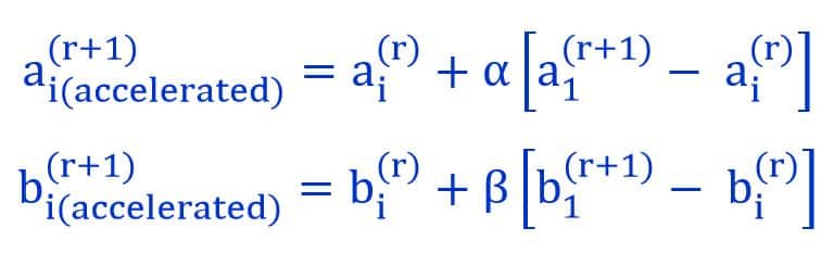
A specific value of the acceleration factor depends upon the system parameters. The optimum value of α is generally in the range of 1.2 to 1.6 for most systems.
Solved problems on Gauss Seidel
Obtain the voltage at bus 2 for the simple system shown in the below Fig, using the GS method, if V1 = 1∠ 00 pu.
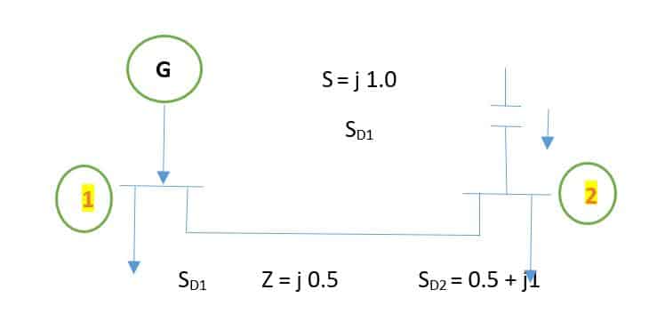
As we can see in the above figure,, the capacitor at bus 2 injects a reactive power of 1.0 pu. At bus 2 the complex power injection is ;
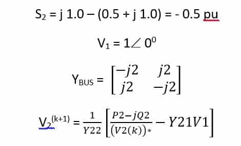
We know that V1 is specified, therefore it will be constant through all iterations.
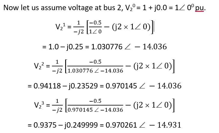
Further, we can simplify the above equation.
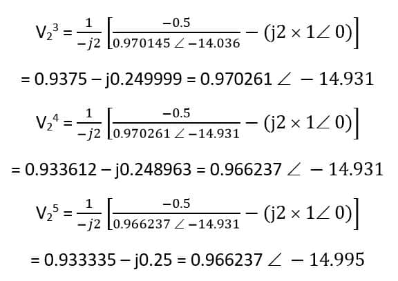
We can stop the iterations now because the difference in the voltage magnitudes is less than 10-6pu,. We can compute the line flow as below,
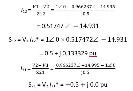
Now the total loss in the line is :
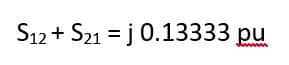
Since the line has no resistance, therefore there is no real power loss.
Read Next